Aggregate Time Series

Time series aggregation rules roll up high-cardinality or high-frequency metrics into pre-aggregated series at ingestion, reducing time series volume before storage. Unlike filtering and sampling, which reduce the number of records, aggregation reduces the volume of a metric: it drops the attributes that fan a metric out into thousands of series and combines the remaining data points into fewer, coarser series.

Time series aggregation applies to metrics. It always runs in Dash0, also for metrics that arrive from a SignalControl Edge collector.

Add an Aggregation Rule

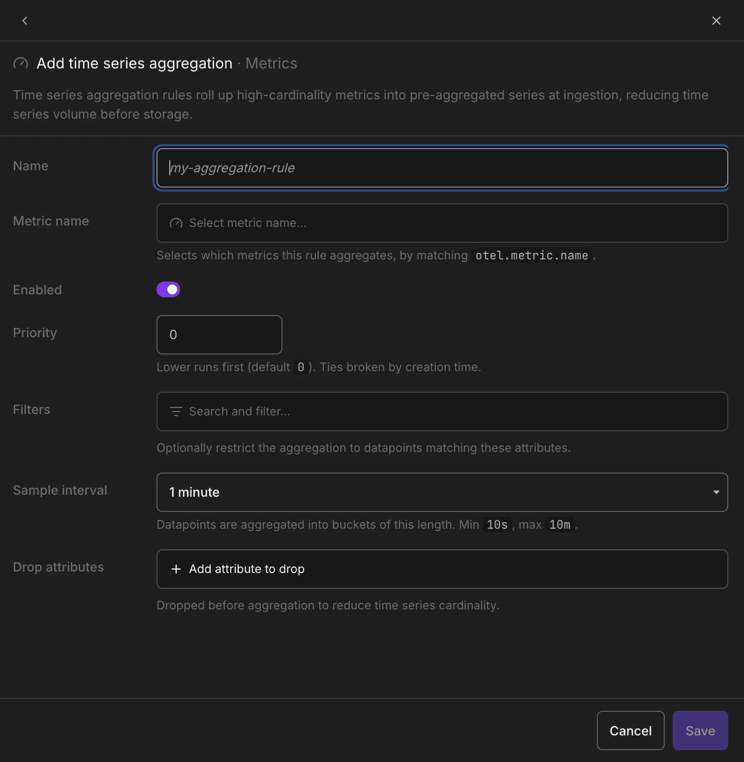
1. From the pipeline, open the Time Series Aggregation stage for Metrics and click Add aggregation rule.
2. Fill in the rule fields:

• Name: A name for the rule, for example my-aggregation-rule.
• Metric name: Selects which metrics the rule aggregates, by matching otel.metric.name.
• Enabled: Activates the rule.
• Priority: Only one rule aggregates a given metric. When several enabled rules match the same metric, the priority decides which one applies: lower runs first (default 0), and ties are broken by creation time. The other matching rules do not run on that metric.
• Filters: Optionally restrict the aggregation to data points matching these attributes.
• Sample interval: Data points are aggregated into buckets of this length. Minimum 10s, maximum 10m.
• Drop scope attributes: Attributes of the instrumentation scope, meaning the library or instrumentation that produced the metric, dropped before aggregation to reduce time series cardinality.
• Drop datapoint attributes: Attributes attached to the individual data points, dropped before aggregation to reduce time series cardinality.

1. Click Save.

How Aggregation Works

Aggregation reduces volume in two ways, which can be combined:

• Spatial aggregation groups data points by attributes. Dropping attributes collapses series that differed only by those attributes into one, reducing cardinality.
• Temporal aggregation groups data points by time. Combining the data points in each Sample interval bucket into a single aggregated data point reduces the frequency of stored data points.

How the values are combined depends on the metric type, so the aggregated series keeps the meaning of the original:

• Gauges: The most recent value wins. Temporal aggregation keeps the latest sample in each bucket, and spatial aggregation keeps the most recently reported value across the series that collapse together.
• Sums (counters): Increments are added up. Cumulative counters are converted to increments first, so combining several counters yields the total across them.
• Histograms and exponential histograms: The bucket counts and totals are merged into one distribution.
• Summaries: Never aggregated. Their quantiles are pre-computed and cannot be merged, so summary metrics pass through unchanged.

Spatial Aggregation

A metric's cardinality is the number of distinct attribute combinations, and each combination is a separate stored time series. Dropping a high-cardinality attribute collapses every series that differed only by that attribute into one.

For example, a request-duration metric split by pod.name, http.method, and http.route produces a series for every combination of the three. If you only chart and alert by route, dropping pod.name and http.method collapses those combinations into one series per route, reducing the stored time series count sharply while preserving the numbers you use.

Temporal Aggregation

Within each Sample interval bucket, the remaining data points for each surviving series are combined into a single aggregated data point, reducing how frequently data points are stored.

Further Reading

• About SignalControl. Overview of the full reduction pipeline and how the stages compose.

• Convert Signals to Metrics. Produce metrics from logs and spans, with attributes set correctly at conversion time.

• Filter Out Spam. Drop noisy records before they reach the aggregation stage.

• Sample Traces. Reduce trace volume while keeping errors and slow traces.