
Last updated: August 21, 2026
What Is Continuous Profiling?
Continuous profiling is the practice of sampling what your code is actually doing on the CPU (and in memory) across your whole fleet, all the time, in production. Instead of running a profiler by hand for a few minutes when something is already on fire, an agent samples the call stacks of every process continuously and ships that data to a backend where you can query it after the fact.
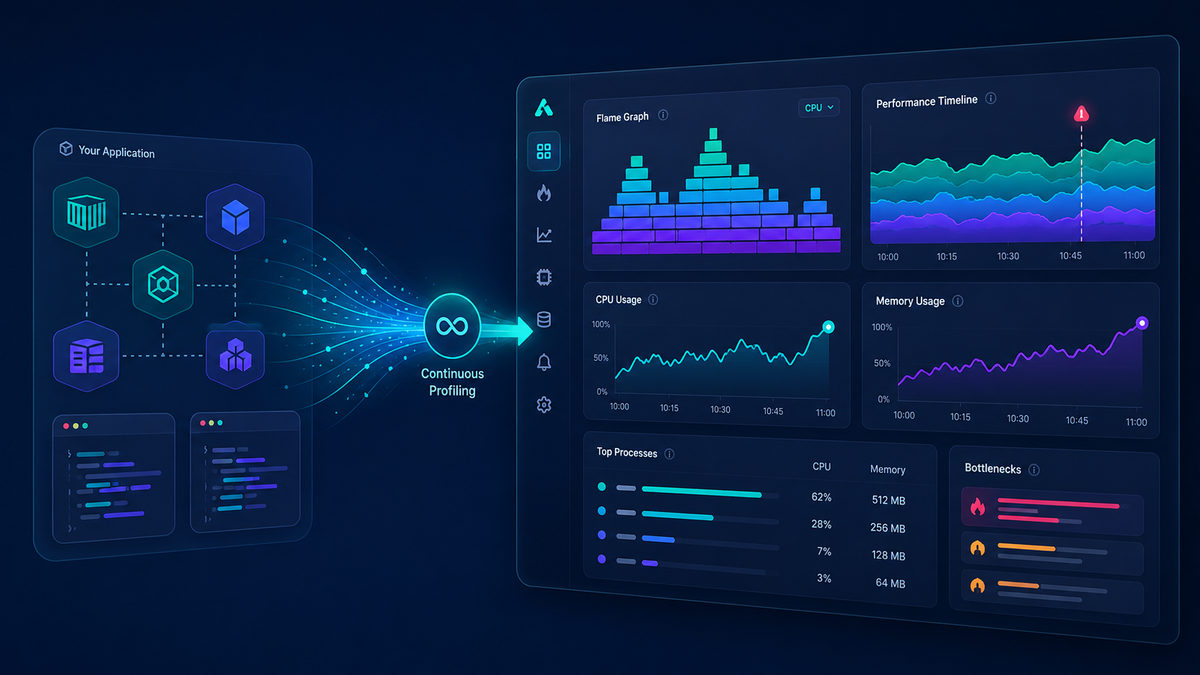 It exists because older profilers were too expensive to leave running. You'd attach one during an investigation, reproduce the problem in staging, and hope the behavior matched production. Continuous profilers flip that around. Sampling-based collection keeps overhead low enough to run permanently (usually a low single-digit percentage of CPU), so the profile is already waiting when you need it. This article covers what continuous profiling measures, how it differs from the signals you already have, how the OpenTelemetry Profiles signal standardizes it, and where the practice bites people.
What continuous profiling actually measures
A profiler answers one question: where is my process spending its resources, down to the line of code? It does this by periodically interrupting the running program (a timer firing at, say, 99 Hz) and recording the current call stack of each thread. Do that thousands of times and the stacks pile up statistically. A function that shows up in 40% of CPU samples is consuming roughly 40% of your CPU time. This is statistical sampling, and it's why the overhead stays low: you're grabbing a snapshot occasionally, not instrumenting every function call.
The usual way to visualize the aggregated result is a flame graph, where the width of each frame is proportional to how often it appeared in the samples. A wide bar near the top is a hot function. A wide tower is a deep, expensive call path.
CPU time is the most common thing to profile, but it isn't the only one. Depending on the runtime and profiler, you can also collect memory allocations, which shows you which code paths are allocating the most and is how you track down heap growth and garbage-collection pressure. You can collect off-CPU time, which shows where threads are blocked waiting on locks, I/O, or syscalls that CPU profiling alone won't surface. Some runtimes also expose lock contention and other runtime events.
How it differs from metrics, logs, and traces
If you already run the three familiar signals, it helps to place profiling next to them precisely, because the boundary with tracing is where most of the confusion lives.
Metrics tell you what changed: CPU usage on this pod jumped at 14:03. Logs tell you what happened: an error was thrown, a request was rejected. Traces tell you where time went across services: this request spent 800ms in the payments service. What none of them tell you is why a given process is burning CPU or allocating memory internally, at the level of individual functions.
Tracing is the one people conflate it with. A trace shows you that a span took 800ms in a service, but it stops at the boundary of your instrumentation. It won't tell you that 600ms of that went into a regex compiled inside a hot loop, unless you happened to wrap that regex in its own span. Profiling fills exactly that gap. It sees the code the tracer never instrumented, because it samples the whole call stack regardless of where you added spans. That's the reason profiling is often called the fourth signal of observability rather than a replacement for any of the existing three.
The real payoff comes from correlation. When a profile sample carries the trace and span ID that was active when it was captured, you can jump from a slow span straight to the functions that made it slow, or from a CPU spike on a metrics dashboard directly into the code responsible for it.
Where OpenTelemetry Profiles fits
Historically every profiling vendor had its own format, which meant your profiling data was locked to whichever tool collected it. OpenTelemetry has been standardizing this with the Profiles signal, the fourth OTLP signal alongside traces, metrics, and logs.
A couple of things about its status are worth pinning down, because competing articles get this wrong. The Profiles signal entered public Alpha in March 2026 and is still under active development. Traces, metrics, and logs are stable in OTLP; profiles are not, and the wire format has already gone through breaking changes. The Profiling SIG originally aimed for strict wire compatibility with Google's pprof format, decided that was impractical, and switched to a convertible model instead. OTLP Profiles is its own format that can round-trip to and from pprof without losing information.
The data model builds on pprof and adds the pieces the rest of OpenTelemetry needs. Each batch carries a Resource and InstrumentationScope, so a profile is attributed to the same service instance as its metrics, logs, and traces. Attributes follow the standard semantic conventions. And a sample can carry a span and trace link, so it points back at the exact request it was captured during.
On the collection side, the reference implementation is an eBPF-based profiler for Linux that Elastic donated to OpenTelemetry. eBPF is what makes whole-system, zero-instrumentation profiling practical: it captures stack traces from the kernel without you modifying or recompiling your applications, and it works across compiled languages that have no runtime profiling hooks. The OpenTelemetry Collector has been able to receive, process, and export profiles since v0.112.0, so the k8sattributesprocessor can tag each profile with the pod and deployment it came from, the same way it does for other signals.
Common pitfalls
Low overhead is not zero overhead, and it isn't uniform. The 1-5% CPU figure you see quoted is an average. A service with very deep call stacks, or one where you've cranked the sampling frequency up, can cost noticeably more. Measure the overhead on your own hot services before you assume the headline number applies to you. Keep the sampling rate sane too; 99 Hz is a common and deliberate choice, because the odd number avoids aliasing with periodic activity in your app.
Symbolization is where profiling quietly breaks. A raw profile is just memory addresses. Turning those into readable function names and line numbers needs debug symbols, and if your production binaries are stripped (as they often are), you either run a symbol server or you spend your afternoon staring at hex. This is the failure that trips up most freshly deployed profilers.
Profiles carry more sensitive data than people expect. Frames contain function names, source file paths, and on some runtimes the local variable names or arguments. In aggregate that discloses your internal code structure, and every so often it leaks a secret or a tenant ID that ended up in a frame argument. If you're exporting profiles to a third-party backend, drop or redact the sensitive frame attributes in the Collector pipeline instead of shipping everything blindly.
Final thoughts
Continuous profiling closes the last gap in production observability. Once you can see which functions are burning CPU and allocating memory, and tie that back to the trace, metric, or log that led you there, root-cause analysis stops at the line of code instead of the service boundary. It's most useful when profiling lives in the same place as your other signals, on the same timeline, rather than in a separate tool you have to context-switch into.
Dash0 supports continuous profiling through the OpenTelemetry eBPF profiler, deployable across your Kubernetes nodes with the Dash0 operator, so profiles land alongside your distributed traces, metrics, and logs and share the same resource context. Because everything sits on one correlated timeline, you can move from a CPU spike on a dashboard to the exact code path behind it without leaving the view.
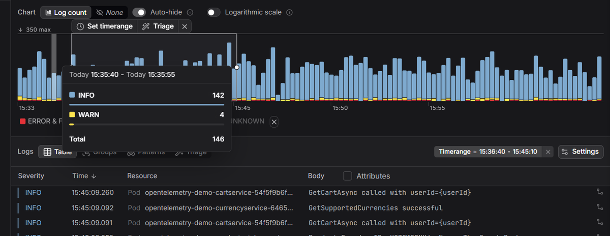 Start a free trial to see your traces, metrics, logs, and profiles correlated in one place. No credit card required.
